Prevalence Of Earthquake Prediction With Reference To Indian Geographical States Through Data Insights

Earthquake sequences exhibit three primary patterns: (1) foreshock-mainshock-aftershock sequences, (2) mainshock-aftershock sequences, and (3) earthquake swarms characterized by the absence of a dominant event [2]. The statistical characterization of these se- quences poses unique challenges for seismic hazard analysis, particularly concerning their temporal distribution.

Foreshocks and aftershocks are generally lower-magnitude events that cluster tempo- rally around a mainshock. This clustering fundamentally violates the Poisson assumption of independent event occurrences. Michael (1997) demonstrated this phenomenon and suggested the use of autoregressive methods to model aftershock sequences [3]. The non- Poissonian nature of earthquake occurrence has prompted the exploration of alternative modeling approaches, such as Markov and semi-Markov processes, as detailed by Anagnos et al (1988) [1].

The temporal scope of aftershock activity remains an area of ongoing research. Utsu (1961) laid the groundwork for understanding magnitude-dependent aftershock duration, and subsequent studies have further refined these temporal parameters [5]. In this study, we conduct a comprehensive analysis of earthquake sequences across all Indian states, employing various methodologies, including truncation, simple clustering, and Omori- Utsu law-based clustering techniques. This multifaceted approach aims to enhance our understanding of seismic activity patterns and improve seismic hazard assessments.

2. Data
   1. Data Collection

The data was collected from the official website of the National Center for Seismology, Ministry of Earth Sciences, Government of India. The dataset contains a complete history of earthquakes that originated in India or neighboring countries during the period from 16-04-2013 to 31-05-2025.

1. 2. Variables in the Dataset

The dataset contains earthquake records with the following key columns:

• • • Timestamp: Date and time of the earthquake (in IST format).
    • Latitude and Longitude: Geographical coordinates of the earthquake.
    • Depth: Depth of the earthquake in kilometers.
    • Magnitude: Earthquake magnitude (e.g., ML, Mb).
    • Location, State, Country: Descriptive location details.
  • Data Processing

Initially, the dataset featured a column named Location, which contained the complete address of the earthquake origin. For the purpose of this study, this column was split into three separate columns:

• • • Country: Identifies the country of origin.
    • State: Denotes the specific state within the country.
    • Location: Describes the region within the state.

This restructuring facilitates clearer insights by categorizing the earthquake data ge- ographically.

As this study exclusively examines earthquakes that originated in India, all instances of earthquakes from neighboring countries have been removed from the dataset. This filtering ensures that the analysis remains pertinent and prevents the introduction of irrelevant data.

To streamline data handling and enable focused analysis, the dataset has been divided into several CSV files. Each file contains the historical records of earthquakes for a single state. This approach improves the organization of the data and allows for state-specific analyses.

All subsequent data processing tasks are conducted in the R programming environment, renowned for its statistical capabilities.

The Magnitude column presented an initial challenge, as it was formatted as alphanu- meric due to the presence of units. This column has been converted into a numeric format to ensure accurate quantitative analysis.

Additionally, a new column titled Interarrival Time has been introduced. This column provides the time interval between successive earthquake occurrences. It is important to note that the calculation of interarrival times is contingent upon the clustering algorithm utilized, which will be discussed further in subsequent sections of this report.

3. Methodology

The process begins with data loading and cleaning. Earthquake data from multiple CSV files are read, ensuring that there is a valid ’time’ column, which is essential for time-based analysis. Timestamps are converted into a standardized datetime format to accommodate various date-time input patterns. Rows with missing or malformed time entries are removed to maintain data integrity. Additionally, magnitude values are sanitized to retain only their numeric components, eliminating any appended text or symbols.

Once the data is cleaned and standardized, the next step involves calculating inter- arrival times—the time intervals between successive earthquake events (specifically, daily maximums, which will be discussed separately). These inter-arrival times are expressed in days and serve as the primary metric for examining the temporal structure of the event sequence.

The Poisson process rate parameter λ is then estimated. It is calculated as the ratio of the total number of earthquake events to the total duration (in days) between the first and last events in the data set. The λ value provides a measure of the average number of events per unit time, which is a key parameter for modeling the events under the Poisson framework.

To validate the assumption of a Poisson process, the study employs the Kolmogorov–Smirnov (KS) test. This test compares the empirical distribution of the calculated inter-arrival times with the theoretical exponential distribution, which is characteristic of inter-arrival times in a Poisson process. A high p-value (typically above 0.05) from the KS test indi- cates a good fit, supporting the hypothesis that the events occur according to a Poisson process. Conversely, a low p-value suggests a deviation from this assumption.

Finally, for each processed dataset, the script records key outcomes, such as the esti- mated Poisson rate (λ), the KS test p-value, and a summary interpretation of the KS test result. These findings are compiled into a master results table and saved to an output CSV file for further analysis and documentation. This methodology ensures a consistent and statistically rigorous assessment of the temporal behavior of earthquake occurrences across multiple datasets.

We tried three different approaches to manage the aftershocks which are described in the coming sections

1. 1. Basic Model

The basic model utilizes a straightforward method for detecting mainshocks. It identifies the most significant earthquake (based on magnitude) that occurs on each calendar day. This is achieved by grouping the dataset by date and selecting the highest-magnitude event from each group. The underlying assumption is that only one important seismic event can occur per day, while any additional events are likely less significant or considered aftershocks. Although this method is computationally efficient and easy to implement, it may oversimplify actual seismic behavior. It does not account for the possibility of two or more independent mainshocks occurring on the same day, particularly in regions with high seismic activity.

1. 2. Clustered Model

While many researchers attempt to predict the time intervals during which aftershocks may occur, there is no definitive rule for determining these periods. However, it is un- derstood that the aftershock period is directly proportional to the magnitude of the mainshock. With this in mind, a clustering rule is defined to manage aftershocks.

The second version adopts a more sophisticated and physically realistic method for identifying mainshocks. It clusters earthquakes based on dynamically assigned time win- dows, which are determined by the magnitude of each potential mainshock. This ap- proach is based on the premise that larger earthquakes tend to produce longer aftershock sequences. For instance, a magnitude 6 earthquake might define a clustering window of ±21 days, whereas a smaller earthquake might only cluster nearby events within ±5 days.

Within each window, the highest-magnitude event is designated as the mainshock, and all surrounding events are considered part of its aftershock sequence. These aftershock windows can be found in [4], and for this study are defined as follows:

This method helps to avoid double-counting related seismic activity and filters out af- tershocks more effectively than the calendar-based approach. However, it comes with increased computational complexity due to the iterative looping and reassignment of events. Despite being more resource-intensive, this version provides a better representa- tion of independent seismic events and aligns more closely with physical seismic models.

1. Truncated Model

Earthquakes with a magnitude less than 5 are generally not felt significantly, and the damage they cause is minimal. Keeping this in mind, the third approach models only destructive earthquakes, which helps manage aftershocks automatically.

In this third version, we introduce a magnitude-based filtering step before identifying mainshocks. Only earthquakes with a magnitude greater than 5 are retained, effectively removing lower-magnitude events and potential noise from the analysis. This step ensures that the dataset focuses solely on moderate to large seismic events, which are more likely to be independent mainshocks rather than aftershocks. After filtering, the code groups the remaining events by the floored date5 and selects the largest magnitude event within each 24-hour period. Although this method resembles the logic of the first version, the critical difference lies in the pre-filtering step: Version 1 considers all events regardless of magnitude, while this version ensures that only significant events are used in the grouping. This approach is efficient and reduces the chance of including aftershocks by eliminating smaller events, but it still assumes that only one important event can occur each day, which could overlook closely timed mainshocks in seismically active regions. Overall, this method offers a practical balance between simplification and relevance by focusing on higher-magnitude data and applying a daily grouping strategy.

2. Omori-Utsu Model

The Omori-Utsu law, also known as the modified Omori law, is a widely recognized empir- ical model in seismology that describes the temporal decay of aftershock activity following a main earthquake event. Initially proposed by Fusakichi Omori in 1894 and later gener- alized by Yoshiro Utsu, the law models how the frequency of aftershocks decreases over time. The mathematical formulation of the Omori-Utsu law is given by:

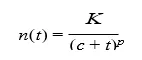
where:

• • • n(t) represents the rate of aftershocks at time t after the mainshock,
    • K is a scaling constant related to the total number of aftershocks,
    • c is a time offset parameter that prevents a singularity at t = 0,
    • p is the decay exponent, typically ranging between 0.9 and 1.5.

This formulation was extensively studied and formalized in the work by Utsu in [5]:

Here we use Omori-Utsu law as a basis for clustering temporally related earthquake events, primarily to identify aftershock sequences. Rather than using the law to fit a time series, it is employed to determine whether two seismic events should be grouped into the same aftershock cluster.

For each earthquake event in a dataset, treated as a potential mainshock, the algo- rithm evaluates all subsequent events. The time difference t (in days) between the current event and each later event is calculated. The Omori-Utsu model is applied to estimate the expected rate of aftershocks at time t:

If n(t) exceeds a threshold, the subsequent event is assigned to the same cluster as the mainshock. This iterative clustering continues through all events in the dataset, assigning a unique identifier Occurrence No to each group.

After clustering, the mainshock of each group is identified as the event with the highest magnitude. The inter-arrival times between these mainshocks are then com- puted. Assuming that these main events follow a Poisson process, the code performs a Kolmogorov–Smirnov (KS) test to evaluate whether the inter-arrival times follow an exponential distribution, which is a key characteristic of a Poisson process.

Further we explored a grid of hyperparameter values for K, c, and p to determine the most appropriate clustering behavior for each file. The KS test is applied for each combi- nation of parameters, and the configuration that yields the highest p-value is considered the best-fitting model. The results are recorded and summarized across all datasets.

4. RESULTS AND INFERENCES

4.1 Basic Model

The results reveal that in 16 out of 29 states, the daily maximum magnitude events appear to follow a Poisson process, suggesting that in these regions, the occurrences of earthquakes are approximately random and independent over time. This is an important finding, as it supports the assumption of statistical regularity in seismicity in a majority of regions.

However, for the remaining 13 states, the data do not conform to the Poisson assump- tion. This deviation is likely due to the presence of aftershock sequences — clusters of events that occur shortly after a larger mainshock — which violate the independence assumption required for a Poisson model. Since this version of the model does not ex- plicitly remove or filter out aftershocks, such correlated events remain in the dataset and distort the temporal randomness expected in a Poisson process. Thus, while the basic model provides a useful first approximation, its limitations in accounting for aftershocks become evident in regions where clustered seismicity is more common.

Compared to the basic static clustering model, which uses fixed temporal or spatial windows to group earthquake events, the Omori-Utsu approach offers significant improve- ments. Static clustering does not adapt to local variations in aftershock decay, which can result in either over-clustering or missing key seismic events. In contrast, the Omori- Utsu model dynamically clusters events using a time-dependent decay law defined by the equation:

where the parameters K, c, and p control the aftershock rate. This approach allows clustering to adjust based on seismicity characteristics specific to each state, leading to more accurate identification of main shocks.

The method also outperforms truncation-based models that classify earthquakes based on a magnitude threshold. Such models assume that only high-magnitude events can be main shocks, which can result in the exclusion of significant lower-magnitude main events, especially in seismically quieter regions. The Omori-based model avoids this bias by considering the temporal relationships between events rather than magnitude alone. This inclusivity ensures that relevant events are retained for analysis and that the derived inter-arrival times more accurately reflect the true underlying process.

Finally, the validation of the model using the Kolmogorov–Smirnov test across all states demonstrates the effectiveness of the Omori-Utsu clustering in extracting a main shock sequence that adheres to the assumptions of a Poisson process. This consistency across diverse seismic environments in India shows the robustness of the method and its potential for use in reliable seismic hazard assessment.

CONCLUSION

This study illustrates the complexities inherent in modeling earthquake occurrences across Indian states. While the Poisson process and subsequent models provide valuable frame- works for understanding seismic behavior, our findings indicate that careful consideration of aftershocks and event magnitudes is critical for accurate representation. The analysis demonstrated that regions exhibiting significant aftershock activity may require tailored approaches to capture the dynamics of seismic events effectively.

The success of the Omori-Utsu model in fitting all states reinforces the importance of adapting modeling techniques to account for temporal decay patterns. Moving forward, it is essential to explore non-Poissonian models and integrate spatial data to enhance predictive accuracy and better inform seismic risk assessments. By developing more so- phisticated and region-specific modeling strategies, we can improve our understanding of earthquake behavior and contribute to more effective disaster preparedness and mitiga- tion efforts.

REFERENCES

1. Thalia Anagnos and Anne S Kiremidjian. A review of earthquake occurrence models for seismic hazard analysis. Probabilistic Engineering Mechanics, 3(1):3–11, 1988.
2. SN Bhattacharya and RS Dattatrayam. Some characteristics of recent earthquake sequences in peninsular india. Gond Geol Magz Spl, 5:67–85, 2003.
3. Andrew J Michael. Testing prediction methods: Earthquake clustering versus the poisson model. Geophysical research letters, 24(15):1891–1894, 1997.
4. United States Geological Survey.    Aftershock forecast overview.   https:// earthquake.usgs.gov/data/oaf/overview.php, 2025. Accessed: 2025-08-13.
5. Tokuji Utsu. A statistical study on the occurrence of aftershocks. Geophys. Mag., 30:521–605, 1961.

REFERENCES

Tirupathi Rao Padi, Sathyala Suresh*, Prevalence Of Earthquake Prediction With Reference To Indian Geographical States Through Data Insights, Int. J. Sci. R. Tech., 2026, 3 (7), 795-804. https://doi.org/10.5281/zenodo.21530234
10.5281/zenodo.21530234