Mathematical Structures In Machine Learning And Neural Networks

Strip away the architecture diagrams and a feedforward neural network is simply a function built by alternating two operations: an affine map (a matrix multiplication plus a bias vector) and a fixed, typically nonlinear, scalar activation function applied coordinate-wise. Training such a network means choosing its parameters to minimize a loss functional measuring the discrepancy between the network's output and the desired output, computed on a finite set of training examples, typically via some variant of gradient descent.

This deceptively simple description raises three distinct mathematical questions, each with its own substantial literature. First, representational capacity: which functions can a network of a given width and depth actually represent, and how does the required size scale with the target accuracy? Second, optimization: given that the loss landscape in parameter space is generally non-convex, why does gradient descent so reliably find good solutions rather than getting stuck? Third, generalization: given that a sufficiently large network can memorize its training data outright, why does it nonetheless perform well on genuinely new inputs? This paper takes each question in turn — Section 3 covers approximation, Section 4 covers optimization via the Neural Tangent Kernel, and Section 5 covers generalization and its more recent geometric reformulation — after Section 2 sets out the basic notation.

2. Networks as Compositional Approximators

A single-hidden-layer network computing a scalar output from an input x ∈ ℝᵈ can be written as in Eq. (1):

f(x) = Σᵢ₌₁ᴺ cáµ¢ σ(wáµ¢·x + báµ¢)           (1)

where σ is the activation function, wáµ¢ and báµ¢ are the weight vector and bias of hidden unit i, and the cáµ¢ are output weights. A deep network of depth L simply nests L such affine–nonlinear layers inside one another. Viewed through the lens of functional analysis, the set of all functions a given architecture can represent is a subset of a function space — typically C(K), continuous functions on a compact set K, under the supremum norm — and the natural question is exactly how large, and how dense, that subset is as width or depth increases.

3. Can the Network Represent What We Want? The Universal Approximation Theorem

3.1 The original result

Cybenko (1989) answered this question for the simplest case: given any continuous sigmoidal σ and any continuous target function f on a compact K ⊂ ℝᵈ, and any tolerance ε > 0, a finite sum of the form of Eq. (1) can be found satisfying Eq. (2):

sup_{x∈K} | f(x) − Σáµ¢ cáµ¢ σ(wáµ¢·x + báµ¢) | < ε (2)

The proof is a density argument: suppose, for contradiction, that the span of functions σ(w·x+b) were not dense in C(K); then, by the Hahn–Banach theorem, some nonzero signed measure would annihilate every function in that span, and Cybenko shows that the specific limiting behaviour of sigmoidal functions rules out the existence of any such measure, forcing density. Hornik, Stinchcombe, and White (1989) reached closely related conclusions independently and extended the result to approximating derivatives as well as function values, and their paper is usually cited jointly with Cybenko's as the origin of the theorem.

3.2 Making it quantitative, and extending it

The 1989 results are existence proofs: they promise a sufficiently wide network exists but say nothing about how wide. Barron (1993) closed part of that gap for functions with an integrable Fourier transform (a smoothness condition), proving the approximation error with N sigmoidal units falls as O(1/√N) — remarkably, independent of the input dimension d, avoiding the curse of dimensionality that plagues many classical approximation schemes.

More recent work extends universal approximation well beyond simple feedforward sigmoidal networks. Wang and Li (2024) formulate a Dynamic Universal Approximation Theorem under which residual convolutional networks and large Transformer-based models are shown to be instances of one common dynamic-approximation framework, in which the function actually computed can depend on the input itself, and use this to design parallelization schemes whose inference time does not grow with depth. Gumaan (2025) proves universal approximation specifically for a single self-attention layer paired with a feed-forward block, showing that even one Transformer layer is, under mild conditions, a universal approximator of sequence-to-sequence maps — a result that helps explain, theoretically, why attention-based architectures underlying today's large language models work as well as they empirically do.

3.3 Seeing it happen

Figure 1 makes the density argument concrete: a fixed target function is fitted by single-hidden-layer sigmoidal networks of increasing width, with output weights obtained by least squares. Growing the network from 3 to 40 hidden units visibly closes the gap between the network's output and the target, a small-scale demonstration of exactly the density property Cybenko (1989) and Hornik et al. (1989) proved abstractly.

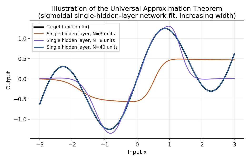
Figure 1. A target function f(x) = sin(2x) + 0.3x approximated by single-hidden-layer sigmoidal networks of width N = 3, 8, and 40, output weights fitted by least squares.

4. Does Training Actually Converge? The Neural Tangent Kernel

Knowing a network can represent the target function says nothing about whether gradient descent, θ_{t+1} = θ_t − η∇L(θ_t), will actually find the parameters that do so — the loss landscape L(θ) is generally riddled with saddle points and local structure in a way that classical convex-optimization theory does not directly address. Jacot, Gabriel, and Hongler (2018) showed that in the limit of infinitely wide networks, this apparent difficulty dissolves: the network's output function evolves under gradient descent exactly as it would under kernel gradient descent with respect to a fixed kernel, the Neural Tangent Kernel (NTK), determined by the architecture and initialization alone and — crucially, in this limit — unchanged throughout training. An ostensibly non-convex training problem thus behaves, in function space, like an ordinary convex kernel regression, for which classical convergence guarantees apply directly.

None of this dispenses with backpropagation (Rumelhart, Hinton, & Williams, 1986), the chain-rule algorithm that actually computes ∇L(θ) efficiently, layer by layer, nor with adaptive optimizers such as Adam (Kingma & Ba, 2015) that remain the practical workhorses of training. What the NTK framework provides is a rigorous, if idealized, account of why gradient descent on this particular non-convex landscape behaves so much better than one might naively expect.

The idealization is not the whole story for realistically sized networks. Chen, Cao, Gu, and Zhang (2020) extend the NTK analysis to noisy gradient descent with weight decay — a more realistic training regime — and derive matching generalization bounds for two-layer networks, while Fort et al. (2020) show empirically that the NTK itself changes rapidly during a short, chaotic initial phase of training before settling down, meaning the strict “frozen kernel” picture only approximately describes what happens in finite, practically sized networks, with most of the useful feature learning concentrated in that early transient.

5. Why Does It Generalize? Classical Bounds and the Geometry of Data

5.1 Counting capacity the classical way

Statistical learning theory, developed principally by Vapnik (1998), answers the generalization question by bounding the gap between training error and true, population-level error in terms of a capacity measure of the hypothesis class — most classically, its Vapnik–Chervonenkis (VC) dimension, a combinatorial count of how many arbitrary point-labelings the class can fit. Bartlett and Mendelson (2002) develop the related, often tighter, Rademacher complexity framework, which measures capacity via the class's ability to correlate with pure noise, yielding generalization bounds that apply directly to neural networks. A long-standing puzzle is that these classical bounds, applied naively to deep networks with vastly more parameters than training examples, predict generalization gaps far larger than what is actually observed — motivating the search, still ongoing, for capacity measures better suited to this heavily over-parameterized regime.

5.2 A geometric answer: data doesn't fill the space it lives in

A complementary explanation appeals to the manifold hypothesis: real-world data — images, audio, language embeddings — is thought to concentrate near a low-dimensional manifold embedded within a much higher-dimensional ambient input space, so the genuine learning problem is far less high-dimensional than the raw input dimension suggests. Bronstein, Bruna, LeCun, Szlam, and Vandergheynst (2017) formalize this as geometric deep learning, arguing that architectures such as convolutional and graph neural networks succeed precisely because they encode geometric priors — translation invariance, permutation invariance, or more general symmetry structure — matched to the intrinsic geometry of the data rather than treating inputs as unstructured Euclidean points. A related body of work on geometric optimization shows that constraining the network's own parameters to a Riemannian manifold, rather than unconstrained Euclidean space, can likewise improve training stability and enforce structural constraints, such as orthogonality, directly through the optimization geometry rather than as an add-on penalty.

CONCLUSION

Three largely independent bodies of mathematics underwrite the practical success of deep learning. Approximation theory, from Cybenko's and Hornik et al.'s original density arguments through to recent universal approximation results for Transformers, establishes that neural networks are expressive enough, in principle, for essentially any task of interest. The Neural Tangent Kernel framework offers a tractable account of why non-convex gradient descent nonetheless reliably converges, at least in the infinite-width idealization, with finite-width analyses filling in a richer, feature-learning picture. Classical statistical learning theory and the newer, geometric, manifold-based perspective together address why over-parameterized networks generalize at all — with the geometric picture offering a particularly compelling account, given that real data is itself far lower-dimensional than its raw representation suggests. Weaving these three strands together into a single, unified mathematical theory of deep learning remains one of the most active open problems in the field.

REFERENCES

1. Barron, A. R. (1993). Universal approximation bounds for superpositions of a sigmoidal function. IEEE Transactions on Information Theory, 39(3), 930–945.
2. Bartlett, P. L., & Mendelson, S. (2002). Rademacher and Gaussian complexities: Risk bounds and structural results. Journal of Machine Learning Research, 3, 463–482.
3. Bronstein, M. M., Bruna, J., LeCun, Y., Szlam, A., & Vandergheynst, P. (2017). Geometric deep learning: Going beyond Euclidean data. IEEE Signal Processing Magazine, 34(4), 18–42.
4. Chen, Z., Cao, Y., Gu, Q., & Zhang, T. (2020). A generalized neural tangent kernel analysis for two-layer neural networks. arXiv:2002.04026.
5. Cybenko, G. (1989). Approximation by superpositions of a sigmoidal function. Mathematics of Control, Signals and Systems, 2(4), 303–314.
6. Fort, S., Dziugaite, G. K., Paul, M., Kharaghani, S., Roy, D. M., & Ganguli, S. (2020). Deep learning versus kernel learning: An empirical study of loss landscape geometry and the time evolution of the neural tangent kernel. arXiv:2010.15110.
7. Goodfellow, I., Bengio, Y., & Courville, A. (2016). Deep learning. MIT Press.
8. Gumaan, E. (2025). Universal approximation theorem for a single-layer Transformer. arXiv:2507.10581.
9. Hornik, K., Stinchcombe, M., & White, H. (1989). Multilayer feedforward networks are universal approximators. Neural Networks, 2(5), 359–366.
10. Jacot, A., Gabriel, F., & Hongler, C. (2018). Neural tangent kernel: Convergence and generalization in neural networks. Advances in Neural Information Processing Systems, 31.
11. Kingma, D. P., & Ba, J. (2015). Adam: A method for stochastic optimization. In Proceedings of the 3rd International Conference on Learning Representations (ICLR).
12. LeCun, Y., Bengio, Y., & Hinton, G. (2015). Deep learning. Nature, 521(7553), 436–444.
13. Rumelhart, D. E., Hinton, G. E., & Williams, R. J. (1986). Learning representations by back-propagating errors. Nature, 323(6088), 533–536.
14. Vapnik, V. N. (1998). Statistical learning theory. Wiley.
15. Vaswani, A., Shazeer, N., Parmar, N., Uszkoreit, J., Jones, L., Gomez, A. N., Kaiser, Ł., & Polosukhin, I. (2017). Attention is all you need. Advances in Neural Information Processing Systems, 30.
16. Wang, W., & Li, Q. (2024). Dynamic universal approximation theory: Foundations for parallelism in neural networks. arXiv:2407.21670.

REFERENCES

Khushal P. Rathod*, Mathematical Structures In Machine Learning And Neural Networks, Int. J. Sci. R. Tech., 2026, 3 (7), 476-479. https://doi.org/10.5281/zenodo.21408506
10.5281/zenodo.21408506